
Precipitation (MSWEP and CHIRPS)#
Product descriptions#
The Multi-Source Weighted-Ensemble Precipitation (MSWEP) is a global precipitation dataset that merges precipitation estimates from a variety of sources into a single gridded product. The MSWEP dataset available in the SALDi Data Cube (SDC) has been acquired from GloH2O with daily, 0.1° (~11 km) resolution.
The product abbreviation used in this package is mswep
The Climate Hazards Group InfraRed Precipitation with Station data (CHIRPS) version 3 product is a 40+ year, high-resolution quasi-global rainfall dataset. Similarly to MSWEP, it combines satellite-based precipitation estimates into a spatially and temporally consistent gridded time series. This product also integrates insitu station data. The CHIRPS dataset available in the SALDi Data Cube (SDC) has been acquired from CHC UCSB with monthly, 0.05° (~5 km) resolution.
The product abbreviation used in this package is chirps
Import packages#
%matplotlib inline
from matplotlib import pyplot as plt
from sdc.load import load_product
Warning
If you use a vector file to load the MSWEP or CHIRPS data, it might happen that the returned xarray DataArray is empty. This can occur when your area of interest is smaller than the pixel size of the dataset and happens to “miss” the nearest pixel center. This is also shortly documented in this issue. To avoid this, you can either test if a larger area of interest works or load data for the entire SALDi site you are working in and then subset the data to your area of interest.
MSWEP example#
mswep = load_product(product="mswep",
                     vec="site06",
                     time_range=("2018-01-01", "2022-01-01"))
mswep
<xarray.DataArray 'precipitation' (time: 1461, latitude: 11, longitude: 13)> Size: 836kB
array([[[2.50000000e-01, 3.75000000e-01, 3.75000000e-01, ...,
         8.75000000e-01, 1.37500000e+00, 1.43750000e+00],
        [2.50000000e-01, 3.12500000e-01, 3.12500000e-01, ...,
         8.75000000e-01, 1.37500000e+00, 1.43750000e+00],
        [1.87500000e-01, 2.50000000e-01, 2.50000000e-01, ...,
         9.37500000e-01, 8.12500000e-01, 8.12500000e-01],
        ...,
        [5.00000000e-01, 6.87500000e-01, 7.50000000e-01, ...,
         1.37500000e+00, 8.12500000e-01, 8.12500000e-01],
        [5.00000000e-01, 7.50000000e-01, 7.50000000e-01, ...,
         1.43750000e+00, 9.37500000e-01, 8.75000000e-01],
        [1.25000000e-01, 1.06250000e+00, 1.12500000e+00, ...,
         1.81250000e+00, 2.25000000e+00, 2.18750000e+00]],

       [[2.31250000e+00, 3.37500000e+00, 3.06250000e+00, ...,
         4.62500000e+00, 7.25000000e+00, 6.68750000e+00],
        [3.56250000e+00, 3.18750000e+00, 3.06250000e+00, ...,
         4.18750000e+00, 5.93750000e+00, 5.62500000e+00],
        [4.25000000e+00, 1.03125000e+01, 5.87500000e+00, ...,
         3.62500000e+00, 4.75000000e+00, 4.93750000e+00],
...
         1.48750000e+01, 1.19453125e+01, 1.27500000e+01],
        [2.98515625e+01, 3.71718750e+01, 3.89609375e+01, ...,
         1.73750000e+01, 1.40546875e+01, 1.43359375e+01],
        [3.26953125e+01, 3.25390625e+01, 3.83437500e+01, ...,
         1.71718750e+01, 1.79921875e+01, 1.90859375e+01]],

       [[4.53125000e-01, 5.07812500e-01, 5.07812500e-01, ...,
         5.46875000e-02, 3.12500000e-02, 3.12500000e-02],
        [4.68750000e-01, 5.00000000e-01, 4.68750000e-01, ...,
         4.68750000e-02, 3.12500000e-02, 3.12500000e-02],
        [1.31250000e+00, 5.07812500e-01, 4.68750000e-01, ...,
         4.68750000e-01, 3.90625000e-02, 3.90625000e-02],
        ...,
        [6.56250000e-01, 5.62500000e-01, 5.78125000e-01, ...,
         1.32812500e-01, 1.40625000e-01, 1.32812500e-01],
        [6.71875000e-01, 5.85937500e-01, 6.17187500e-01, ...,
         1.48437500e-01, 1.48437500e-01, 1.40625000e-01],
        [8.90625000e-01, 8.75000000e-01, 9.14062500e-01, ...,
         6.25000000e-02, 2.57812500e-01, 2.50000000e-01]]],
      shape=(1461, 11, 13), dtype=float32)
Coordinates:
  * time         (time) datetime64[ns] 12kB 2018-01-01 2018-01-02 ... 2022-01-01
  * latitude     (latitude) float32 44B -24.95 -25.05 -25.15 ... -25.85 -25.95
  * longitude    (longitude) float32 52B 30.85 30.95 31.05 ... 31.85 31.95 32.05
    spatial_ref  int32 4B 4326
Attributes:
units: mm d-1In comparison to other datasets, the MSWEP data is not loaded lazily, so you see the underlying numpy array when displaying the data. Notice the low spatial resolution (0.1° = ~11 km) of the data. The entire SALDi site 06 is covered by only 143 pixels:
mswep.shape[1] * mswep.shape[2]
143
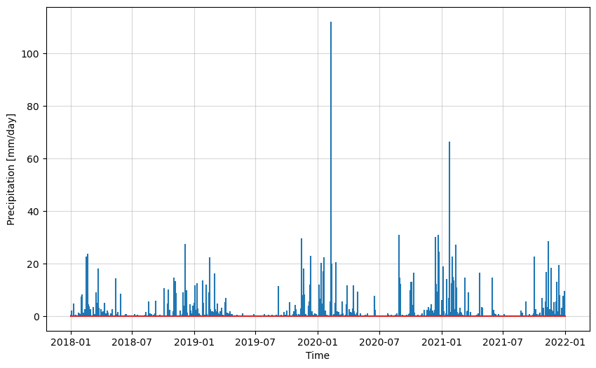
As an example, let’s plot the precipitation for a point using a Matplotlib stem plot:
mswep_pt = mswep.sel(longitude=31.5384, latitude=-25.0226, method="nearest")
fig, ax = plt.subplots(figsize=(10, 6))
ax.stem(mswep_pt.time, mswep_pt, markerfmt="")
ax.grid(True, alpha=0.5)
plt.xlabel("Time")
plt.ylabel("Precipitation [mm/day]")
Text(0, 0.5, 'Precipitation [mm/day]')
Tip
Even Stackoverflow threads that are more than 9 years old can be helpful sometimes 🙂: https://stackoverflow.com/questions/26042735/python-matplotlib-stem-plot-with-no-markers
CHIRPS example#
CHIRPS data is available for a 40+ year period, so let’s load all data available for the same site to calculate long-term statistics. Don’t worry about loading too much data. Because of the low resolution and monthly time step, the total data size in this case is only about 1.2 MB.
chirps = load_product(product="chirps", vec="site06")
chirps
<xarray.DataArray (time: 528, latitude: 22, longitude: 26)> Size: 1MB
array([[[360.373   , 381.25592 , 393.65714 , ..., 163.71133 ,
         161.91153 , 149.72266 ],
        [372.7863  , 417.43408 , 414.54425 , ..., 163.38391 ,
         162.06677 , 153.17998 ],
        [396.18085 , 425.69714 , 430.05145 , ..., 166.52878 ,
         167.24496 , 159.05054 ],
        ...,
        [207.82388 , 219.655   , 226.3153  , ..., 168.29129 ,
         178.21489 , 199.62668 ],
        [188.18501 , 224.67062 , 240.18958 , ..., 173.59999 ,
         191.61238 , 209.27744 ],
        [170.63715 , 180.17308 , 201.83875 , ..., 167.0087  ,
         190.08994 , 208.32477 ]],

       [[230.4233  , 258.13226 , 278.1335  , ..., 131.31548 ,
         131.24693 , 136.31024 ],
        [236.85828 , 273.16693 , 287.68823 , ..., 134.94858 ,
         136.34167 , 146.70804 ],
        [235.17365 , 267.10657 , 282.76196 , ..., 112.51571 ,
         115.5153  , 120.03358 ],
...
        [147.03372 , 152.8964  , 148.74081 , ...,  81.440765,
          77.7007  ,  86.26249 ],
        [136.0836  , 155.33276 , 151.62842 , ...,  88.969696,
          80.11787 ,  90.20367 ],
        [126.51878 , 133.8095  , 125.29382 , ...,  75.45819 ,
          88.892914,  88.60953 ]],

       [[155.83394 , 159.77188 , 172.3072  , ...,  77.4873  ,
          76.84388 ,  78.05698 ],
        [162.0739  , 185.19853 , 174.8246  , ...,  76.233055,
          78.209785,  72.60957 ],
        [169.4051  , 174.95306 , 186.82559 , ...,  75.13494 ,
          75.36551 ,  79.64299 ],
        ...,
        [225.47302 , 233.80696 , 235.98016 , ..., 115.94058 ,
         107.69514 , 102.9259  ],
        [222.71065 , 248.35959 , 255.15381 , ..., 103.38594 ,
         105.601845, 106.1416  ],
        [213.41785 , 228.1623  , 221.60959 , ...,  77.07419 ,
          97.32357 , 100.948944]]], shape=(528, 22, 26), dtype=float32)
Coordinates:
  * time         (time) datetime64[ns] 4kB 1981-01-01 1981-02-01 ... 2024-12-01
  * latitude     (latitude) float64 176B -24.93 -24.98 -25.03 ... -25.93 -25.98
  * longitude    (longitude) float64 208B 30.78 30.83 30.88 ... 31.98 32.03
    band         int64 8B 1
    spatial_ref  int32 4B 4326
Attributes:
    TIFFTAG_DOCUMENTNAME:      /home/CHIRPS/v3.0/monthly/africa/chirps-v3.0.1...
    TIFFTAG_IMAGEDESCRIPTION:  IDL TIFF file
    TIFFTAG_SOFTWARE:          IDL 8.9.0, L3Harris Geospatial Solutions, Inc.
    TIFFTAG_DATETIME:          2024:11:27 16:57:13
    TIFFTAG_XRESOLUTION:       100
    TIFFTAG_YRESOLUTION:       100
    TIFFTAG_RESOLUTIONUNIT:    2 (pixels/inch)
    AREA_OR_POINT:             Area
    scale_factor:              1.0
add_offset: 0.0print(f"Data size: {chirps.nbytes / 1e6} MB")
Data size: 1.208064 MB
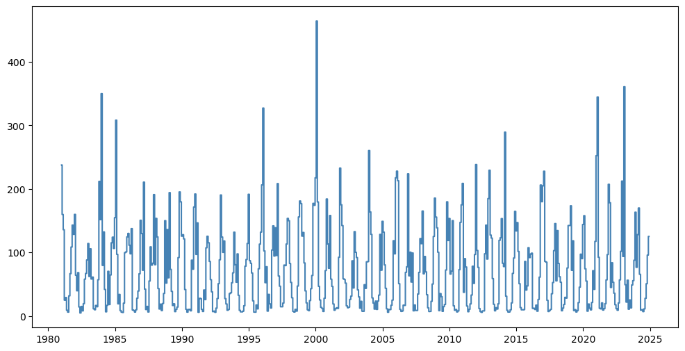
We first aggregate the data spatially by calculating the mean value per time step across the entire site:
chirps_mean_xy = chirps.mean(dim=["longitude", "latitude"])
As an alternative to the stem plot shown earlier, Matplotlib’s step plot is also well suited to visualize precipitation time series:
fig, ax = plt.subplots(figsize=(12, 6))
ax.step(x=chirps_mean_xy.time,
        y=chirps_mean_xy,
        where='mid', color='steelblue')
plt.show()
chirps_mean_xy_subset = chirps_mean_xy.sel(time=slice("2018-01-01", "2024-12-31"))
fig, ax = plt.subplots(figsize=(12, 6))
ax.grid(which='both', linestyle='-', linewidth=0.25)
ax.axhline(0, color='gray', linewidth=.5, linestyle='-') # plot a thicker line at y=0
ax.step(x=chirps_mean_xy_subset.time,
        y=chirps_mean_xy_subset,
        where='mid', color='steelblue')
plt.title('Monthly precipitation for SALDi site 6 (2018-2024)')
plt.ylabel('Precipitation [mm/month]')
plt.show()

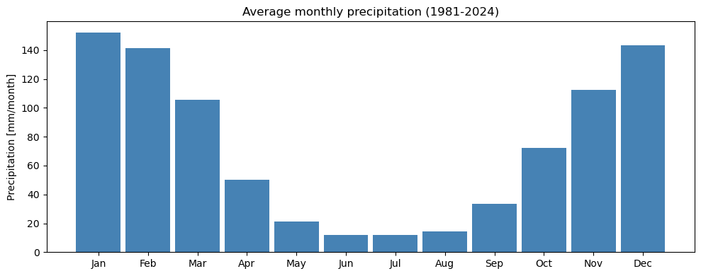
One interesting long-term statistic is the average monthly precipitation over the entire period of record. This can be calculated by grouping the data by month and calculating the mean for each month. We thereby get 12 values representing the long-term average precipitation for each month of the year:
chirps_long_term_monthly_mean = chirps_mean_xy.groupby('time.month').mean(dim='time')
chirps_long_term_monthly_mean
<xarray.DataArray (month: 12)> Size: 48B
array([152.28539 , 141.45778 , 105.80175 ,  50.31505 ,  21.254389,
        11.827967,  12.148655,  14.229453,  33.329124,  72.44721 ,
       112.53735 , 143.33305 ], dtype=float32)
Coordinates:
  * month        (month) int64 96B 1 2 3 4 5 6 7 8 9 10 11 12
    band         int64 8B 1
    spatial_ref  int32 4B 4326
Attributes:
    TIFFTAG_DOCUMENTNAME:      /home/CHIRPS/v3.0/monthly/africa/chirps-v3.0.1...
    TIFFTAG_IMAGEDESCRIPTION:  IDL TIFF file
    TIFFTAG_SOFTWARE:          IDL 8.9.0, L3Harris Geospatial Solutions, Inc.
    TIFFTAG_DATETIME:          2024:11:27 16:57:13
    TIFFTAG_XRESOLUTION:       100
    TIFFTAG_YRESOLUTION:       100
    TIFFTAG_RESOLUTIONUNIT:    2 (pixels/inch)
    AREA_OR_POINT:             Area
    scale_factor:              1.0
add_offset: 0.0fig, ax = plt.subplots(figsize=(10, 4))
plt.bar(x=chirps_long_term_monthly_mean.month - 1,
height=chirps_long_term_monthly_mean,
width=0.9,
color='steelblue',
align='center')
plt.title('Average monthly precipitation (1981-2024)')
plt.ylabel('Precipitation [mm/month]')
plt.xlabel(None)
month_names = ['Jan', 'Feb', 'Mar', 'Apr', 'May', 'Jun', 'Jul', 'Aug', 'Sep', 'Oct', 'Nov', 'Dec']
plt.xticks(ticks=range(12), labels=month_names, rotation=0)
plt.tight_layout()
plt.show()
Based on this long-term monthly mean, we can calculate monthly anomalies by subtracting the long-term monthly mean from the original time series. This way, we get a time series that shows how much wetter or drier each month was compared to the long-term average for that month:
chirps_long_term_monthly_anomalies = chirps_mean_xy.groupby('time.month') - chirps_long_term_monthly_mean
chirps_long_term_monthly_anomalies_subset = chirps_long_term_monthly_anomalies.sel(time=slice("2018-01-01", "2024-12-31"))

fig, ax = plt.subplots(figsize=(10, 4))
ax.grid(which='both', linestyle='-', linewidth=0.25)
ax.axhline(0, color='gray', linewidth=.5, linestyle='-') # plot a thicker line at y=0
ax.step(x=chirps_long_term_monthly_anomalies_subset.time,
        y=chirps_long_term_monthly_anomalies_subset,
        where='mid', color='steelblue')
plt.title('Monthly precipitation anomaly based on long-term mean (1981-2024)')
plt.ylabel('Precipitation anomaly [mm/month]')
plt.tight_layout()
plt.show()
To make the anomalies more comparable (e.g., between regions), the standard deviation of the long-term monthly anomalies can be calculated and used to normalize the anomalies. This way, we get a time series of standardized anomalies that shows how many standard deviations each month was above or below the long-term average for that month. You can find an example in this notebook.