Sentinel-1 RTC#
Product description#
The Sentinel-1 Radiometric Terrain Corrected (RTC) data product available in the SALDi Data Cube (SDC) is a mirror of Digital Earth Africa’s product of the same name.
Detailed information can be found here and here.
The product abbreviation used in this package is s1_rtc
Import packages#
%matplotlib inline
from matplotlib import pyplot as plt
import numpy as np
from sdc.load import load_product
Loading data#
ds = load_product(product="s1_rtc",
                  vec="site06",
                  time_range=("2021-01-01", "2022-01-01"))
ds
[WARNING] Loading data for an entire SALDi site will likely result in performance issues as it will load data from multiple tiles. Only do so if you know what you are doing and have optimized your workflow! It is recommended to start with a small subset to test your workflow before scaling up.
<xarray.Dataset> Size: 98GB
Dimensions:      (latitude: 5500, longitude: 6500, time: 211)
Coordinates:
  * latitude     (latitude) float64 44kB -24.9 -24.9 -24.9 ... -26.0 -26.0 -26.0
  * longitude    (longitude) float64 52kB 30.75 30.75 30.75 ... 32.05 32.05
    spatial_ref  int32 4B 4326
  * time         (time) datetime64[ns] 2kB 2021-01-01T03:17:55.709725 ... 202...
Data variables:
    vv           (time, latitude, longitude) float32 30GB dask.array<chunksize=(211, 563, 563), meta=np.ndarray>
    vh           (time, latitude, longitude) float32 30GB dask.array<chunksize=(211, 563, 563), meta=np.ndarray>
    area         (time, latitude, longitude) float32 30GB dask.array<chunksize=(211, 563, 563), meta=np.ndarray>
angle (time, latitude, longitude) uint8 8GB dask.array<chunksize=(211, 1127, 1127), meta=np.ndarray>Exactly as the example in the Sentinel-2 L2A notebook, we have now lazily loaded Sentinel-1 RTC data. If you are not familiar with the concept of lazy loading, please refer to Xarray, Dask and lazy loading and the Sentinel-2 L2A notebook. The latter also covers some Xarray basics (Look for the “Xarray Shorts” sections), so be sure to check it out if you haven’t already!
Let’s have a closer look at the vh-band (vertical transmit, horizontal receive):
ds.vh
<xarray.DataArray 'vh' (time: 211, latitude: 5500, longitude: 6500)> Size: 30GB
dask.array<vh, shape=(211, 5500, 6500), dtype=float32, chunksize=(211, 563, 563), chunktype=numpy.ndarray>
Coordinates:
  * latitude     (latitude) float64 44kB -24.9 -24.9 -24.9 ... -26.0 -26.0 -26.0
  * longitude    (longitude) float64 52kB 30.75 30.75 30.75 ... 32.05 32.05
    spatial_ref  int32 4B 4326
  * time         (time) datetime64[ns] 2kB 2021-01-01T03:17:55.709725 ... 202...
Attributes:
nodata: nanConverting to decibel scale#
With Synthetic Aperture Radar (SAR) data, it is often useful to convert the data
to decibel (dB) scale for visualization purposes. The Sentinel-1 RTC data here is stored
in power (linear) scale by default and can be converted to decibel scale using numpy’s
log10-method
and multiply the result by 10:
vh_db = 10 * np.log10(ds.vh)
vh_db
<xarray.DataArray 'vh' (time: 211, latitude: 5500, longitude: 6500)> Size: 30GB
dask.array<mul, shape=(211, 5500, 6500), dtype=float32, chunksize=(211, 563, 563), chunktype=numpy.ndarray>
Coordinates:
  * latitude     (latitude) float64 44kB -24.9 -24.9 -24.9 ... -26.0 -26.0 -26.0
  * longitude    (longitude) float64 52kB 30.75 30.75 30.75 ... 32.05 32.05
    spatial_ref  int32 4B 4326
  * time         (time) datetime64[ns] 2kB 2021-01-01T03:17:55.709725 ... 202...
Attributes:
nodata: nanWarning
Due to the logarithmic nature of the decibel scale, it is not appropriate for some mathematical operations. For example, the mean of decibel data is not the same as the mean of the data in power (linear) scale. It is recommended to keep the data in power (linear) scale for your analysis and only convert to decibel scale for visualization purposes in the end.
Tip
The SAR Handbook is a great resource on topics related to SAR data processing and interpretation. Regarding power vs decibel scale, have a closer look at Chapter 3 Tutorial and the sections “Comparing histograms of the amplitude, power, and dB scaled data” (p. 92) and “Why is the scale important?” (p. 93) in particular.
Notice how the data structure above is still the same as for the
vh-band we started with and that the data is still lazily loaded. The only
difference is the increase of graph layers in the row called “Dask graph”. Dask
is constructing a graph behind the scenes, which is a representation of the
computation that will be executed once the data is loaded into memory.
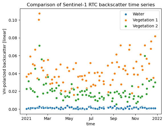
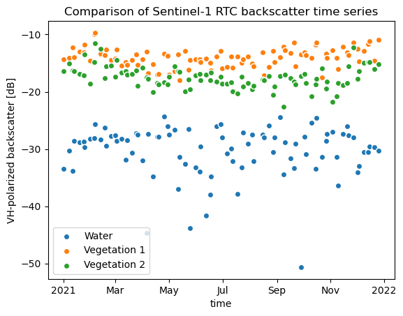
To see the difference between the power and the decibel scaled data, let’s plot the time series of Xarray Shorts: Indexing and basic plotting again:
px_water = (31.571, -24.981)
px_veg1 = (31.5384, -25.0226)
px_veg2 = (31.551, -25.034)

vh_px_water = ds.vh.sel(longitude=px_water[0], latitude=px_water[1], method="nearest")
vh_px_veg1 = ds.vh.sel(longitude=px_veg1[0], latitude=px_veg1[1], method="nearest")
vh_px_veg2 = ds.vh.sel(longitude=px_veg2[0], latitude=px_veg2[1], method="nearest")

vh_db_px_water = vh_db.sel(longitude=px_water[0], latitude=px_water[1], method="nearest")
vh_db_px_veg1 = vh_db.sel(longitude=px_veg1[0], latitude=px_veg1[1], method="nearest")
vh_db_px_veg2 = vh_db.sel(longitude=px_veg2[0], latitude=px_veg2[1], method="nearest")
vh_px_water.plot.scatter(x="time", label="Water")
vh_px_veg1.plot.scatter(x="time", label="Vegetation 1")
vh_px_veg2.plot.scatter(x="time", label="Vegetation 2")
plt.title("Comparison of Sentinel-1 RTC backscatter time series")
plt.ylabel("VH-polarized backscatter [linear]")
plt.legend()
<matplotlib.legend.Legend at 0x7f10230ddaf0>

vh_db_px_water.plot.scatter(x="time", label="Water")
vh_db_px_veg1.plot.scatter(x="time", label="Vegetation 1")
vh_db_px_veg2.plot.scatter(x="time", label="Vegetation 2")
plt.title("Comparison of Sentinel-1 RTC backscatter time series")
plt.ylabel("VH-polarized backscatter [dB]")
plt.legend()
<matplotlib.legend.Legend at 0x7f10230bfe00>

Xarray Shorts: Groupby-operations#
Combining groupby-operations
with aggregation functions can be very useful to calculate statistics for
different time periods. In the following example, we calculate the median for
each month of the year.
Let’s first just apply the groupby-operation. The result is a xarray.core.groupby.DataArrayGroupBy
object, which is a lazy representation of the grouped data.
vh_monthly = ds.vh.groupby("time.month")
vh_monthly
<DataArrayGroupBy, grouped over 1 grouper(s), 12 groups in total:
    'month': 12 groups with labels 1, 2, 3, 4, 5, 6, 7, 8, 9, 10, 11, 12>
Tip
Handling Xarray’s datetime components as in the example above can be very useful. You can find an overview on this topic here.
We can now apply an aggregation function to the grouped data. In this case, we
calculate the median for each month of the year. The result is a
xarray.DataArray object with a new month-dimension.
Notice that the size of the array is now much smaller than the original vh
data we started with because we have reduced the number of time steps from 211
(acquisitions) to 12 (months). The size is an estimate of the potential memory
footprint of the data.
vh_monthly_median = vh_monthly.median(dim="time")
vh_monthly_median
<xarray.DataArray 'vh' (month: 12, latitude: 5500, longitude: 6500)> Size: 2GB
dask.array<stack, shape=(12, 5500, 6500), dtype=float32, chunksize=(1, 563, 563), chunktype=numpy.ndarray>
Coordinates:
  * latitude     (latitude) float64 44kB -24.9 -24.9 -24.9 ... -26.0 -26.0 -26.0
  * longitude    (longitude) float64 52kB 30.75 30.75 30.75 ... 32.05 32.05
    spatial_ref  int32 4B 4326
  * month        (month) int64 96B 1 2 3 4 5 6 7 8 9 10 11 12
Attributes:
nodata: nanWe could have also chained both operations together, which would have resulted in the same output:
vh_monthly_median = ds.vh.groupby("time.month").median(dim="time")
You can find an overview of which methods are available for grouped
DataArrayGroupBy objects here.
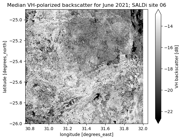
As you can probably imagine, these operations can be very useful to handle and analyse large time series data. Instead of going further at this point, let’s just convert the result to decibel scale, select the month of June and plot it:
vh_monthly_median_db = 10 * np.log10(vh_monthly_median)
vh_monthly_median_db.sel(month=6).plot(robust=True, cmap="gray", cbar_kwargs={"label": "VH backscatter [dB]"})
plt.title("Median VH-polarized backscatter for June 2021; SALDi site 06")
Text(0.5, 1.0, 'Median VH-polarized backscatter for June 2021; SALDi site 06')

